Research Methods and Professional Practice - Exercises

Research Methods and Professional Practice - Exercises
This site contains exercices and practitces that were part of the Module Research Methods and Professional Practice.
📚 Table of Contents
- Unit 7: Hypothesis Testing and Summary Measures Worksheet
- Unit 8: Charts Worksheet and Analysis
- References
Unit 7: Hypothesis Testing and Summary Measures Worksheet
These exercises introduce key statistical summary measures in Excel, such as the mean, standard deviation, median, and quartiles, using real dietary data. You will analyse weight loss for two diets and interpret which appears more effective based on these statistics.
7.1.1B - Descriptive Statistics and Data Exploration
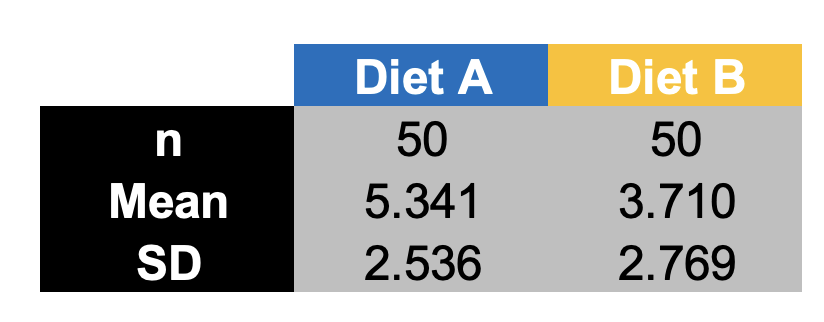 Figure 1: Exercise 7.1.1B (University of Essex Online, 2025)
Key Findings
- Measured on the Mean and Standard Diviation, the data implies that Diet B is less effective.
7.1.2B - Frequency Distributions
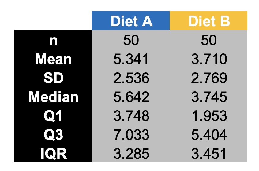 Figure 2: Exercise 7.1.2B (University of Essex Online, 2025)
Key Findings
- The Median confirms the Mean.
- Diet A has a slight left skew.
- For Diet B, the Mean almost identical to the Median.
- Dieat A has a Q1 of 3.7 while Diet B has a Mean of 3.7. This means 75% of paticipians from Diet A scored higher than the average person from Diet B.
7.1.3B - Comparative Analysis of Distributions
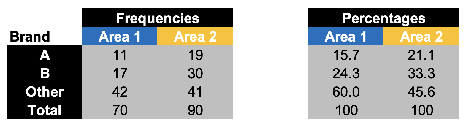 Figure 3: Exercise 7.1.3B (University of Essex Online, 2025)
Key Findings
- Both Areas have Other as the preferred cereal brand.
- Area 1 has Other as most chosen brand.
- Area 2 has more active or diverse distribution of Cereal A and B compared to Area 1.
7.2.2 - Filtration Agent Comparison (Paired t-Test)
 Figure 4: Exercise 7.2.2 (University of Essex Online, 2025)
Key Findings
- We are testing if Agent 1 is more effective (lower impurity).
- Null Hypothesis ($H_0$): $\mu_1 \ge \mu_2$ (Agent 1 is not more effective; the mean difference is zero or positive).
- Alternative Hypothesis ($H_1$): $\mu_1 < \mu_2$ (Agent 1 is more effective; impurity levels are strictly lower).
- Mean Difference: $-0.43$ (Agent 1 is lower on average)
- One-tailed p-value: $0.0038$
- The one-tailed p-value ($0.0038$) is significantly lower than the standard alpha level of $0.05$. Therefore, we reject the null hypothesis. There is strong statistical evidence to conclude that Filter Agent 1 is more effective than Filter Agent 2 at removing impurities.
7.2.3 - Income Comparison by Gender
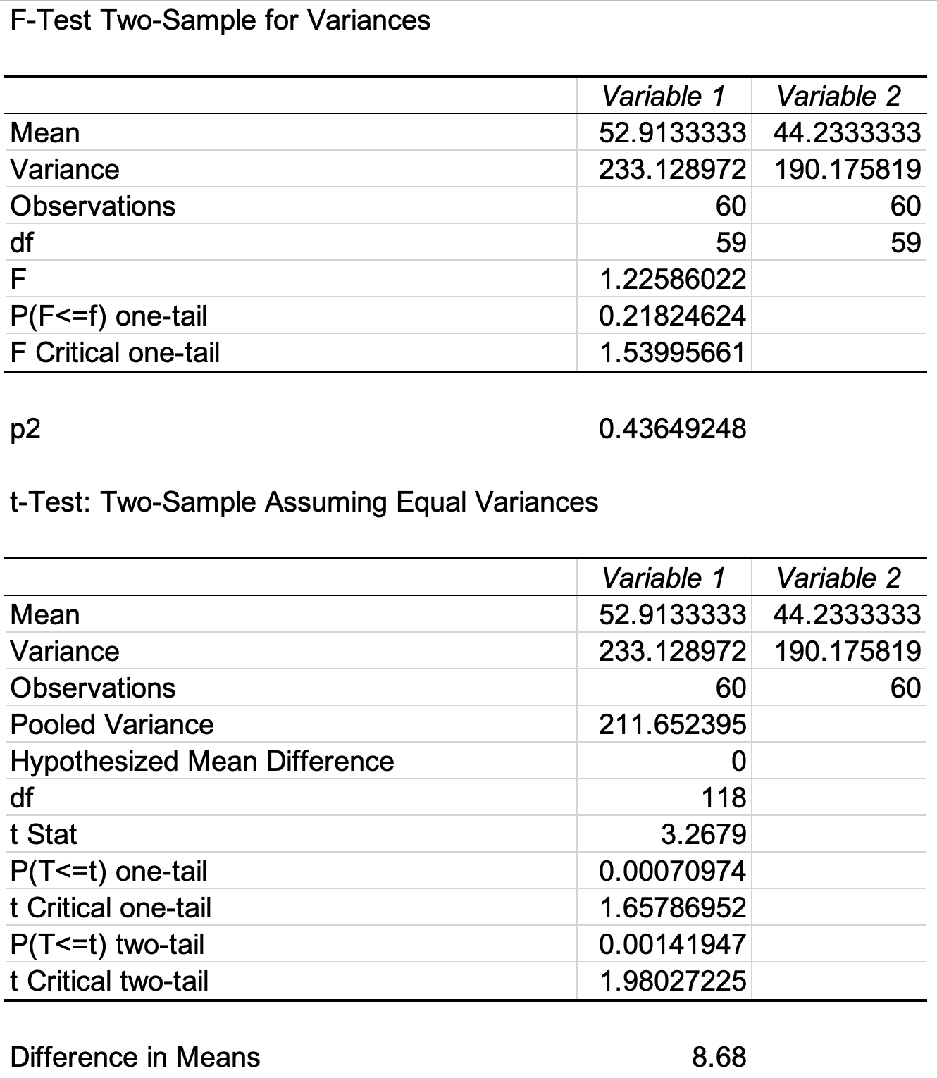 Figure 5: Exercise 7.2.3 (University of Essex Online, 2025)
Key Findings
Check: Homogeneity of Variance
- Null Hypothesis ($H_0$): \(\sigma^2_{\text{male}} = \sigma^2_{\text{female}}\) (The variances are equal).
- Alternative Hypothesis ($H_1$): \(\sigma^2_{\text{male}} \neq \sigma^2_{\text{female}}\) (The variances are different).
- F-Statistic: $1.23$
- P-value: $0.436$
- Since the p-value ($0.436$) is greater than the significance level ($\alpha = 0.05$), we fail to reject the null hypothesis. Hence we can proceede with the t-Test.
t-Test
- Null Hypothesis ($H_0$): \(\mu_{\text{male}} \le \mu_{\text{female}}\) (Male income is not significantly greater than female income).
- Alternative Hypothesis ($H_1$): \(\mu_{\text{male}} > \mu_{\text{female}}\) (Male income is significantly greater than female income).
- The analysis shows that the mean income for males (£52,910) is higher than for females (£44,230). The difference of £8,680 is statistically significant ($t = 3.27$, $p < .001$).
- Verdict: We reject the null hypothesis. There is strong evidence to conclude that the population mean income for male cardholders exceeds that of female cardholders.
7.2.4 - Comparison of Filtration Agents
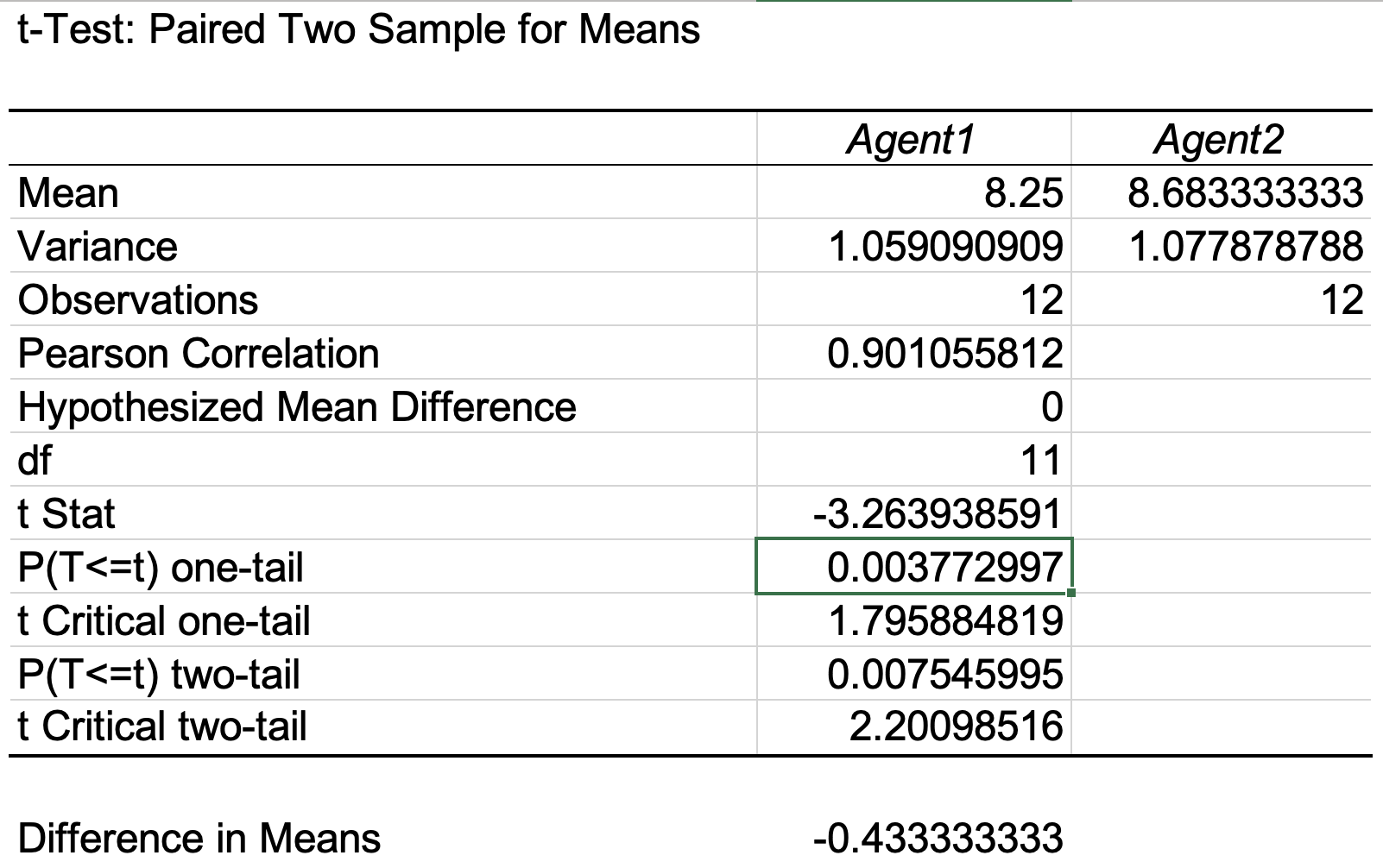 Figure 6: Exercise 7.2.4 (University of Essex Online, 2025)
Key Findings
- Null Hypothesis ($H_0$): $\mu_1 = \mu_2$ (There is no difference in effectiveness between the two agents).
- Alternative Hypothesis ($H_1$): $\mu_1 \neq \mu_2$ (There is a significant difference in effectiveness).
- The analysis shows a mean difference of -0.43 units between the two agents. The probability of observing such a difference (or larger) by random chance is approximately 0.8% ($p = 0.0075$).
- Since $p < 0.05$, we reject the null hypothesis.
- Verdict: There is a statistically significant difference in the effectiveness of the two filtration agents. Specifically, Agent 1 results in significantly lower impurity levels ($M=8.25$) than Agent 2 ($M=8.68$).
7.2.5 - Gender and Income Comparison
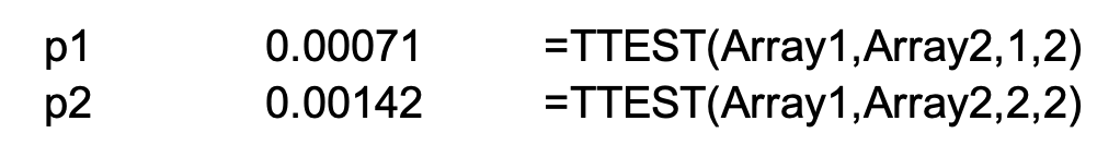 Figure 7: Exercise 7.2.5 (University of Essex Online, 2025)
Key Findings
- Null Hypothesis ($H_0$): \(\mu_{\text{male}} \le \mu_{\text{female}}\) (Male income is less than or equal to female income).
- Alternative Hypothesis ($H_1$): \(\mu_{\text{male}} > \mu_{\text{female}}\) (Male income is strictly higher than female income).
- The statistical test returns a p-value of 0.0007.
- Because $p < 0.05$, the result is highly significant. Hence we reject the null hypothesis.
- Verdict: There is strong statistical evidence to conclude that the population mean income for males exceeds that of females.
Unit 8: Charts Worksheet and Analysis
These exercises introduce the use of bar charts and histograms in Excel to summarise and compare real-world data on brands, habitats and diets.
8.1 - Brand Preference by Area
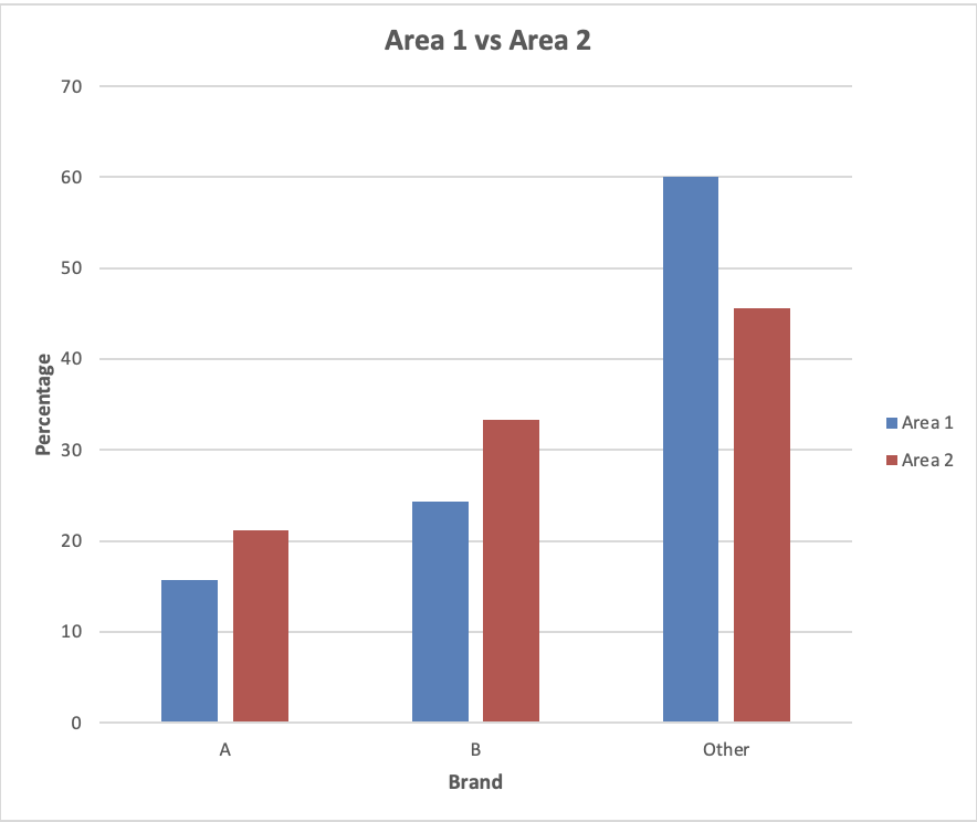 Figure 8: Exercise 8.1 (University of Essex Online, 2025)
Key Findings
- The charts show that “Other” is the most preferred brand in both areas, but its dominance is noticeably stronger in Area 1 (60%) than in Area 2 (about 45%).
- In Area 2, both A and B gain a larger share (just over half of all preferences combined), suggesting a more competitive brand environment where the manufacturer’s brands are more actively chosen and the “Other” category is less overwhelming than in Area 1.
8.2 - Heathland Location A vs B
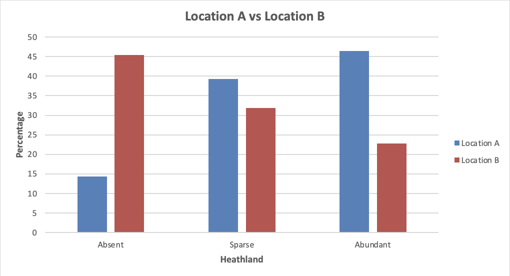 Figure 9: Exercise 8.2 (University of Essex Online, 2025)
Key Findings
- The heather species is much more established in Location A, where almost half the transects are classed as Abundant and only a small minority as Absent.
- In Location B, the species is often absent and only rarely abundant, indicating a considerably poorer level of colonisation.
- Overall, the distribution shifts from “mostly abundant” in Location A to “mostly absent or sparse” in Location B, showing a clear ecological contrast between the two heathlands.
8.3 - Diet A vs B
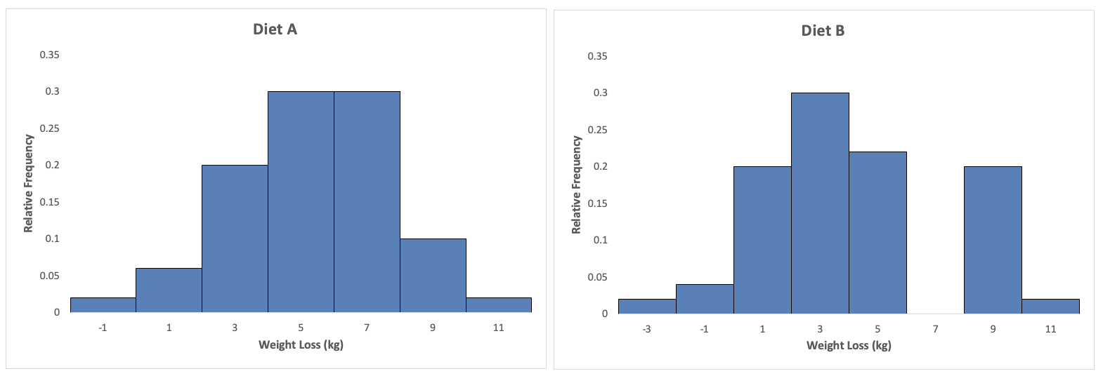 Figure 10: Exercise 8.3 (University of Essex Online, 2025)
Key Findings
- Both diets produce a wide range of outcomes, but Diet A’s weight loss values cluster more tightly around moderate to high losses (around 4–8 kg), suggesting more consistent performance.
- Diet B shows a more uneven spread, with some participants gaining weight or losing very little and a few achieving quite high losses, indicating greater variability in response.
- Overall, the histograms suggest that Diet A tends to deliver more reliably positive weight loss, whereas Diet B appears less predictable, with both poorer and very strong individual results.
References
- University of Essex Online (2025) Unit 7: Inferential Statistics and Hypothesis Testing. Available at: https://www.my-course.co.uk/course/view.php?id=14231§ion=13 (Accessed 10 December 2025)
- University of Essex Online (2025) Unit 8: Data Analysis and Visualisation. Available at: https://www.my-course.co.uk/course/view.php?id=14231§ion=14 (Accessed 10 December 2025)